How to perform a thermal stress analysis

The temperature distribution in a part can cause thermal stress effects (stresses caused by thermal expansion or contraction of the material).  Examples of this phenomenon include interference fit processes (also called shrink fits), where parts are mated by heating one part and keeping the other part cool for easy assembly.  Another example is thermal creep, which is permanent deformation resulting from prolonged application of a stress below the elastic limit.  An example of this is the behavior of metals exposed to mechanical loads and elevated temperatures over time.

Thermal stress effects can be simulated by coupling a heat transfer analysis (steady-state or transient) and a structural analysis (static stress with linear or nonlinear material models or Mechanical Event Simulation [MES]).  The process consists of two basic steps:

1. Perform a heat transfer analysis to determine the temperature distribution.
2. Directly input the temperature results as a load in a structural analysis to determine the stress and displacement caused by the temperature loads.

For example, a thermal stress analysis of a transistor and heat sink assembly was performed as follows:

• A steady-state heat transfer analysis was performed to obtain the temperature distribution (see Figure 1).

Figure 1:  A transistor and heat sink model with temperature distribution results from a steady-state heat transfer analysis.

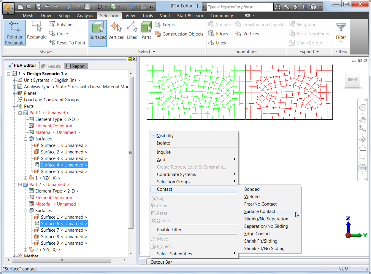
• In the FEA Editor environment of Autodesk Simulation Mechanical, the analysis type was changed for a structural analysis.  In this case, static stress with linear material models was used.
• Constraints were specified for the structural analysis by fully fixing the two bottom surfaces of the model.  Additional structural loads (such as forces, pressures, and gravity) could have been added if desired; however, for this example, the only loads were the temperatures from the heat transfer analysis.
• On the "Multipliers" tab of the "Analysis Parameters" dialog, a load case multiplier of "1" was specified in the "Thermal" column so that thermal effects would be included in the structural analysis (see Figure 2).

Figure 2:   A load case multiplier was specified to include thermal effects in the structural analysis.

• On the "Thermal" tab of the "Analysis Parameters" dialog, "Another Design Scenario in loaded file" was chosen from the pull-down menu of options in the "Source of temperatures" field.  "1 – Design Scenario 1" was chosen from the pull-down menu of options in the "Use temperatures from Design Scenario" field was used to specify the location of the temperature results file from the previous steady-state heat transfer analysis (see Figure 3).

Figure 3:   The "Thermal" tab of the "Analysis Parameters" dialog was used to specify the Design Scenario that would be used as input to the static stress analysis with linear material models.

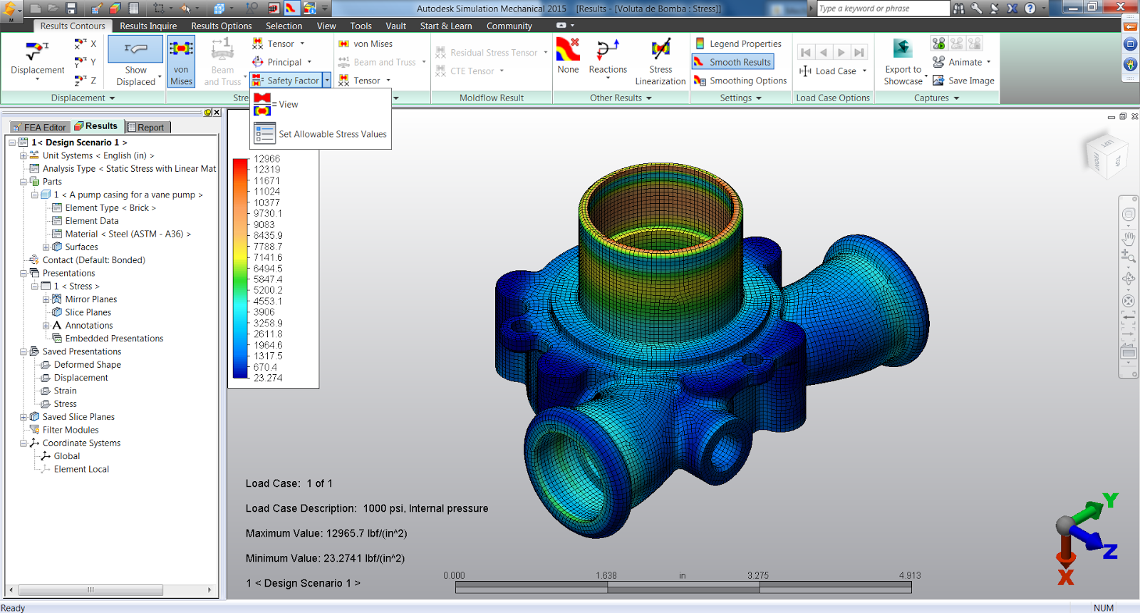
• The static stress analysis with linear material models was run and then the results, including thermal stress effects, were displayed in the Results environment (see Figure 4).

Figure 4:   Displacements (left) and stresses (right) in the transistor and heat sink assembly due to temperature loads, displayed in the Results environment.

Thus, the ability to couple heat transfer and structural analysis capabilities provides an easy and convenient way to simulate thermal stress effects. 

How to Determine the Factor of Safety

When evaluating the results of a linear static stress analysis, one can specify allowable stress values and then display factor of safety contours to see where stresses in the model are below and above those allowables. Viewing factor of safety contours can help one decide whether a design needs modification or is acceptable and is ready for manufacturing.

To display factor of safety contours, choose the "View" command in the "Safety Factor" dropdown of the “Stress” panel in the “Results Contours” tab of Autodesk Simulation (see Figure 1).

Figure 1: In the "Safety Factor" dropdown, choose the "View" command to display factor of safety contours.

When this command is activated, color-coded contours of the factor of safety for the selected stress contour will be shown (see Figure 2).

Figure 2: In the Results environment, one can specify allowable stress values and then display factor of safety contours. This contour shows a color-coded graphical display of where stresses in the model are below and above the specified allowables.

The factor of safety is the ratio of the allowable stress to the actual stress:

• A factor of safety of 1 represents that the stress is at the allowable limit.
• A factor of safety of less than 1 represents likely failure.
• A factor of safety of greater than 1 represents how much the stress is within the allowable limit.

The allowable stresses can be assigned on a per part basis by choosing the "Set Allowable Stress Values" command in the "Safety Factor" dropdown (see Figure 3).

Figure 3: Choose the "Set Allowable Stress Values" command in the "Safety Factor" dropdown to specify allowable stress values.

The "Allowable Stress Values" dialog will appear and each part will be listed in a separate row. One can specify a value in the "Allowable Stress" column or press the "Load Yield Stress" or "Load Ultimate Stress" buttons to load the values from the material library (see Figure 4). Any parts for which the allowable stress is set to 0 will be excluded from the factor of safety calculations.

Figure 4: In the "Allowable Stress Values" dialog, one can enter a value for a part in the "Allowable Stress" column or press the "Load Yield Stress" or "Load Ultimate Stress" buttons to load the values from the material library.

Thus, the ability to view factor of safety contours helps engineers determine what the results say about the adequacy of a design. For example, examining these contours can help you properly exercise engineering judgment when balancing between material cost reduction and ensuring a safe product.

How to define a local coordinate system

When setting up a model for analysis, it can be easier and more efficient to add loads and constraints in a coordinate system other than the default (particularly for off-axis loads or constraints or for curved geometry). The FEA Editor environment of Autodesk Simulation Mechanical provides the ability to define local coordinate systems (rectangular, cylindrical, or spherical with the origin located anywhere in space) and then add loads and constraints relative to them.

For example, consider a model with a cylindrical surface. To define the vector for a tangential edge force you can no longer use the global coordinate system. You will need to define a local coordinate system and use it to define your load vector.

Define a cylindrical local coordinate about the centerline of the cylinder as follows:

• In the FEA Editor environment tree view, right click on "Coordinate Systems" to access a pop-up menu of options and choose "New..."  The "Creating Coordinate System Definition" dialog will appear (see Figure 1).  This screen provides options for defining a new coordinate system.

Figure 1: The "Creating Coordinate System Definition" dialog is used to define local coordinate systems.

• Click on the "Coordinate System Type" field and choose from the pull-down menu of options.  For this example, "Cylindrical" was specified.
• Enter three sets of coordinates in the "Point A", "Point B" and "Point C" fields to define the local coordinate system per the diagram shown on the screen. 
• Alternatively, you can define coordinates by clicking on points in the model as follows:
• Click on the “Select A,” “Select B,” or “Select C” button.  Then click on a vertex in the model to define the coordinate.
• Click on the "Interactive" button. Then click on three vertices to define all three points sequentially. A graphical display of an axis will be drawn on the model to guide you as you click on the points.
• Click on the "OK" button to accept the coordinate system definition. It will then be listed in the model tree under "Coordinate Systems".

Now, you can conveniently add a force load to the model relative to the local coordinate system. 

For this example, select the edges and right click anywhere in the working area to access a pop-up menu of options. Choose "Coordinate Systems" and then the local cylindrical coordinate system to apply it to the selected edges (see Figure 2). Icons indicating the orientation of the local cylindrical coordinate system will appear on the vertices.

Figure 2: Apply the local cylindrical coordinate system to the selected edges

Right click in the working area and choose "Add" and "Edge Forces..." to access the "Creating Nodal Force Objects" dialog. Notice that the active local cylindrical coordinate system is shown in the "Coordinate System" field (see Figure 3). The axis icons on the selected vertices will indicate the direction that you should define for the force load. In this case, the Y direction was specified to designate the tangential direction.

Figure 3:  Add a force load to the selected Edges. The active local cylindrical coordinate system is shown in the "Coordinate System" field

After adding the force load, the display will show the force arrows pointing in relation to the local cylindrical coordinate system (see Figure 4).

Figure 4: The force load is applied in relation to the local cylindrical coordinate system

Thus, defining a local coordinate system in the FEA Editor can make it easier to apply loads and constraints. Local coordinate systems can either be reused in the Results environment or defined there to display results in an arbitrary orientation relative to them

How to simulate rising levels of water over time in FEA

In a time based analysis (MES) Hydrostatic pressure is a straight forward load you can apply to any surface within Simulation Mechanical. All you have to do is to;

• pick a surface,
• define the direction of gravity (which will increase the pressure load linearly in that direction) and
• enter the fluid density

But what if you wanted to simulate effects of increase in the amount of water over time?  

Think of heavy rains over a short period of time and its effects on a dam gate like the one shown here.

Hydrostatic pressure load definition does not give you the option to change the water level over time. 

No need to panic J

Instead of increasing the water level, you can simply use prescribed displacements to move the object deeper and deeper in to the water which will increase the pressure acting on the surface.

To accomplish this I recommend creating 2 load curves:

• The 1^st one will be ramp up style and it will control the motion.
• The 2^nd one will be a steady load curve and it will control the hydro static pressure.
• Make sure the hydrostatic pressure you have applied has the “follows displacement” option enabled. 

When you run the simulation you will see that the deformations will increase as your design dips deeper in to the water which represents rising water levels. 

The video on the right shows the increase in stress levels as the pressure builds up

How and When to Take Advantage of Symmetry and Antisymmetry

When creating a model for finite element analysis, natural lines of symmetry and antisymmetry can allow you to analyze a structure or system by modeling only a portion of it. This technique can reduce the size of the model (the total number of nodes and elements), which can reduce the analysis run time as well as the demands on computer resources.

Symmetry

Symmetry means a model is identical on either side of a dividing line or plane (see Figures 1-3). Along the line or plane of symmetry, boundary conditions must be applied to represent the symmetrical part as follows:

• Out-of-plane displacement = 0
• The two in-plane rotations = 0

Figure 1: Model with a Line of Symmetry

Figure 2: Model with a Plane of Symmetry

Figure 3: Example of Symmetry for Plate Elements

Antisymmetry

Antisymmetry means the loading of a model is oppositely balanced on either side of a dividing line or plane (see Figures 4-5). Boundary conditions must be applied along the line of symmetry as follows:

• Out-of-plane rotation = 0
• The two in-plane displacements = 0

Figure 4: Antisymmetrical Model

Figure 5: Example of Antisymmetry for Plate Elements

Figure 6 shows an example of how to specify an antisymmetrical boundary condition in Autodesk Simulation Mechanical software.

Figure 6: Defining an Antisymmetrical Boundary Condition

Required Conditions

To take advantage of the symmetrical modeling technique, the following conditions for symmetry (or antisymmetry) must exist:

• the geometry, material properties and boundary conditions are symmetric; and
• the loading is symmetric or antisymmetric.

Then, you can build a model of the symmetrical portion (half, quarter, eighth, etc.) and apply the appropriate boundary conditions.

Advantages of a symmetrical/antisymmetrical model include the following:

• Analyzing a symmetrical portion of a structure means faster processing than if you modeled the whole structure.
• You can often increase the mesh density of the symmetrical model for greater accuracy and still have fewer elements than if you modeled the whole structure.
• You can compare the results of a symmetrical model to those of a full model to confirm the validity

How to sum reaction forces

The summation of reaction forces in a model is often used to verify input loading, validate model behavior or determine floor load distributions. In the Results environment, the "Inquire: Results" dialog can be used to sum the reaction forces of selected nodes.

Another typical application of summing reaction forces is to determine the total force of a pressure load when the area of pressure is unknown and cannot be readily calculated. As shown in Figure 1, the cutting frame has a pressure load applied to two surfaces of unknown area and is fully constrained at the bottom of each of the four legs. The total force of the pressure can be calculated by summing the vertical reactions of all of the constrained nodes.

Figure 1: Note the locations of the pressure loads and constraints in this display of the vertical reaction forces in the cutting frame.

To sum the reaction forces in the Results environment for a Static Stress Analysis:

• Select and display the desired reaction (X, Y or Z) using the "Results Contours” tab,  “Other Results” panel, “Reactions” pull-down menu “Reaction Force (Negative) ” pull-out menu;
• Select the nodes that will be used in the summation;
• Right click anywhere in the working area;
• In the pop-up menu that appears, select "Inquire Results"; and
• In the "Inquire: Results" dialog (Figure 2), click on the "Summary" pull-down menu and select "Sum".

Figure 2: The "Inquire: Results" dialog displays information about the selected nodes and the calculated "Summary" value.

The summary of the reaction forces of all selected nodes will now be displayed in the "Inquire: Results" dialog. If desired, the area could be calculated since the pressure and force values are now known.

Understanding Degrees of Freedom

For finite element analysis (FEA) users, it's important to keep in mind that some types of elements might not transmit all types of loads through their nodes. For example, two structural beam elements connected together behave like a fully welded connection because the beam elements will transmit three forces (axial and two shears) and three moments (torsion and two bending). However, a beam element connected to a truss element behaves like a pinned joint because the truss element can only transmit axial forces. The concept of what forces are transmitted and consequently what loads and restraints can be applied is known as degree of freedom (DOF).

The DOF is important to understand in determining how loads can be applied, how boundary conditions restrain the model and how different element types need to be connected together. A translational DOF indicates that forces are transmitted through the nodes and a rotational DOF indicates that moments are transmitted through the nodes.

For example, two-dimensional (2-D) elements only have translational DOFs. Thus, you cannot apply a nodal moment to a 2-D element; mathematically, the element cannot react to the moment.

Figure 1: 2D Elements (Triangular)		Figure 2: 2D Elements (Quadrilateral)

In addition, a "fully fixed" boundary condition cannot provide a moment restraint to a brick element because brick elements only have translational DOFs.

Figure 3: Brick Elements (8 noded)

Finally, the beam to truss element connections could be unstable because the truss element will not prevent the beam element from rotating; if the other end of the beam is free to translate, then the connection behaves like a ball joint.

Figure 4: Beam Element to Truss Element connection

The last two examples may result in model stability messages (such as "model not tied down enough") during a linear static stress analysis.

Table 1: DOFs for common structural element types.

Element	Degrees of Freedom
Truss	translation in X, Y, Z
Beam	translation in X, Y, Z; rotation in X, Y, Z
2-D	translation in Y, Z
Brick	translation in X, Y, Z
Plate	translation in X, Y, Z; Two in-plane rotation DOFs (The out-of-plane rotational DOF is not considered for plate elements)

Note: This is a small subset of the available element types in Autodesk Simulation Mechanical software, see the User's Guide for a full list.

How to define surface contact in 2D analyses

For linear static stress analysis of two-dimensional (2-D) assembly models that are created using Autodesk Simulation’s sketching, modeling and meshing capabilities, you can conveniently and quickly define contact between parts. To do so, use the following general method:

1. Sketch the 2-D parts (the parts must share at least one identical-length, coincident edge).
2. Select the sketches in the tree view and click on the “Generate 2D Mesh” button within the “Mesh” panel under the “Mesh” tab (see Figure 1). The "2-D Mesh Generation" dialog will appear.

Figure 1: In the tree view, select the sketches that share a coincident edge and then click “Generate 2D Mesh” to access the "2D Mesh Generation" command.

3. Adjust the mesh settings as necessary and press “Apply” to generate the mesh.
4. In the model display, select the coincident surfaces and right click. In the pop-up menu, choose "Contact" and then specify the type of contact from five applicable options (see Figure 2):
• Bonded - The nodes on the two edges will be matched and will be in perfect contact throughout the analysis. When a node on one edge deflects, the node on the adjoining edge will deflect the same amount in the same direction. This is the default option.
• Free/No Contact - The nodes on the two edges will not be matched and will be free to move relative to each other.
• Surface Contact - The nodes on the two edges will be matched and will be free to move away from each other. If the nodes move toward each other, a stiffness will be applied to resist this movement.

o   Sliding/No Separation – Bonds contact faces in normal to face direction while sliding under deformation.

o   Separation/No Sliding – Separates contact faces partially or fully without them sliding against each other.

Note that Edge Contact and Welded Contact are not applicable to 2D elements.

Figure 2: Once the mesh is generated, you can select and right click on the coincident surfaces and specify the type of contact.

4. After defining the type of contact, the contact surfaces will be listed in the tree view.
5. In the tree view, right click on the contact pair and choose "Settings..." (see Figure 3).

Figure 3: Right click on the contact pair in the tree view and choose "Settings...".

6. In the "Contact Options" dialog, you can specify the coefficient of friction for the contact pair (see Figure 4).

Figure 4: Choose whether or not to include friction in the analysis and specify the static friction coefficient.

7. Set up for linear static stress analysis (define element information, material properties, loadings and constraints) and run the analysis.
8. In the Results environment, you can inquire on the total contact force for each contact pair in the model. Right click on the heading for the contact pair in the tree view and choose the "Contact Force..." command (see Figure 5).

Figure 5: In Results environment, you can inquire on the total contact force. A "Total Contact Force" dialog will appear with the total contact force for that pair.

Thus, the ability to quickly and easily define 2-D contact helps you to perform linear static stress analysis of 2-D assembly models that were created with Autodesk Simulation’s sketching, modeling and meshing tools.