Viewing applied temperatures

If you are concerned about thermally induced stresses in your design, you will want to run a thermal analysis to determine the temperature distribution. Then, map the temperature results to a subsequent structural analysis.

Mechanical Event Simulation (MES) allows a user to apply such temperatures automatically, whether from a steady-state or transient heat transfer analysis.

If you have previously run a transient thermal analysis, you may want to ensure that the mapping algorithm used for transferring the temperatures to an MES analysis has worked as expected. After all, you could be using different mesh sizes for each analysis type, and the nodal temperatures may not map one-to-one from a transient thermal analysis to an MES analysis.

So how do you check if the mapping was done correctly?

Here is how:

In this example, the FEM file is located in the following folder (C:\FEA\Bracket.fem)

Let’s say that, in Design Scenario 1, you conducted a Transient Heat Transfer analysis on an Assembly using a 100% mesh size. 

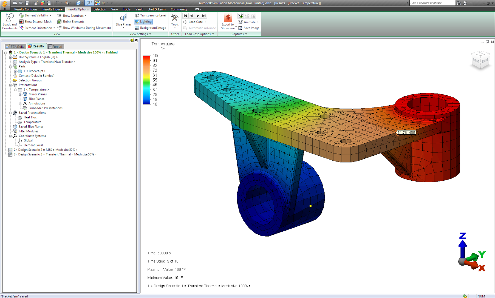
Then, you created a second Design Scenario as an MES analysis and meshed it with a 50% mesh size. You then applied the thermal loads within the Thermal tab of the Analysis Parameters dialog. 

Before running the MES analysis, simply perform a “Check Model” operation. This action creates the solid mesh and decodes the geometry, loads, and constraints. If you look in the Design Scenario 2 folder (C:\FEA\Bracket.ds_data\2), you will now see a file named “ds_map.tto”, which is a transient temperature output file mapped from Design Scenario 1 to Design Scenario 2.

At this point, change the analysis type from MES to Transient Thermal, creating a 3^rd Design Scenario. Keep the same mesh size (50%) as used in the MES analysis.

Using Windows Explorer, copy the file “ds_map.tto” from “C:\FEA\Bracket.ds_data\2” to “C:\FEA\Bracket.ds_data\3”.  Then, rename the copied file “ds.tto” (deleting “_map” from the name).

Within Simulation Mechanical perform a “Check Model” operation for the 3^rd design scenario, which is the second transient thermal analysis, without applying any loads or constraints. 

In the Results environment for design scenario 3, you will now be able to see the temperature results that were mapped from Design Scenario 1 (utilizing a 100% mesh size) to Design Scenario 2 (utilizing a 50% mesh size).   

How and When to Take Advantage of Symmetry and Antisymmetry

When creating a model for finite element analysis, natural lines of symmetry and antisymmetry can allow you to analyze a structure or system by modeling only a portion of it. This technique can reduce the size of the model (the total number of nodes and elements), which can reduce the analysis run time as well as the demands on computer resources.

Symmetry

Symmetry means a model is identical on either side of a dividing line or plane (see Figures 1-3). Along the line or plane of symmetry, boundary conditions must be applied to represent the symmetrical part as follows:

• Out-of-plane displacement = 0
• The two in-plane rotations = 0

Figure 1: Model with a Line of Symmetry

Figure 2: Model with a Plane of Symmetry

Figure 3: Example of Symmetry for Plate Elements

Antisymmetry

Antisymmetry means the loading of a model is oppositely balanced on either side of a dividing line or plane (see Figures 4-5). Boundary conditions must be applied along the line of symmetry as follows:

• Out-of-plane rotation = 0
• The two in-plane displacements = 0

Figure 4: Antisymmetrical Model

Figure 5: Example of Antisymmetry for Plate Elements

Figure 6 shows an example of how to specify an antisymmetrical boundary condition in Autodesk Simulation Mechanical software.

Figure 6: Defining an Antisymmetrical Boundary Condition

Required Conditions

To take advantage of the symmetrical modeling technique, the following conditions for symmetry (or antisymmetry) must exist:

• the geometry, material properties and boundary conditions are symmetric; and
• the loading is symmetric or antisymmetric.

Then, you can build a model of the symmetrical portion (half, quarter, eighth, etc.) and apply the appropriate boundary conditions.

Advantages of a symmetrical/antisymmetrical model include the following:

• Analyzing a symmetrical portion of a structure means faster processing than if you modeled the whole structure.
• You can often increase the mesh density of the symmetrical model for greater accuracy and still have fewer elements than if you modeled the whole structure.
• You can compare the results of a symmetrical model to those of a full model to confirm the validity

How to sum reaction forces

The summation of reaction forces in a model is often used to verify input loading, validate model behavior or determine floor load distributions. In the Results environment, the "Inquire: Results" dialog can be used to sum the reaction forces of selected nodes.

Another typical application of summing reaction forces is to determine the total force of a pressure load when the area of pressure is unknown and cannot be readily calculated. As shown in Figure 1, the cutting frame has a pressure load applied to two surfaces of unknown area and is fully constrained at the bottom of each of the four legs. The total force of the pressure can be calculated by summing the vertical reactions of all of the constrained nodes.

Figure 1: Note the locations of the pressure loads and constraints in this display of the vertical reaction forces in the cutting frame.

To sum the reaction forces in the Results environment for a Static Stress Analysis:

• Select and display the desired reaction (X, Y or Z) using the "Results Contours” tab,  “Other Results” panel, “Reactions” pull-down menu “Reaction Force (Negative) ” pull-out menu;
• Select the nodes that will be used in the summation;
• Right click anywhere in the working area;
• In the pop-up menu that appears, select "Inquire Results"; and
• In the "Inquire: Results" dialog (Figure 2), click on the "Summary" pull-down menu and select "Sum".

Figure 2: The "Inquire: Results" dialog displays information about the selected nodes and the calculated "Summary" value.

The summary of the reaction forces of all selected nodes will now be displayed in the "Inquire: Results" dialog. If desired, the area could be calculated since the pressure and force values are now known.

How to define surface contact in 2D analyses

For linear static stress analysis of two-dimensional (2-D) assembly models that are created using Autodesk Simulation’s sketching, modeling and meshing capabilities, you can conveniently and quickly define contact between parts. To do so, use the following general method:

1. Sketch the 2-D parts (the parts must share at least one identical-length, coincident edge).
2. Select the sketches in the tree view and click on the “Generate 2D Mesh” button within the “Mesh” panel under the “Mesh” tab (see Figure 1). The "2-D Mesh Generation" dialog will appear.

Figure 1: In the tree view, select the sketches that share a coincident edge and then click “Generate 2D Mesh” to access the "2D Mesh Generation" command.

3. Adjust the mesh settings as necessary and press “Apply” to generate the mesh.
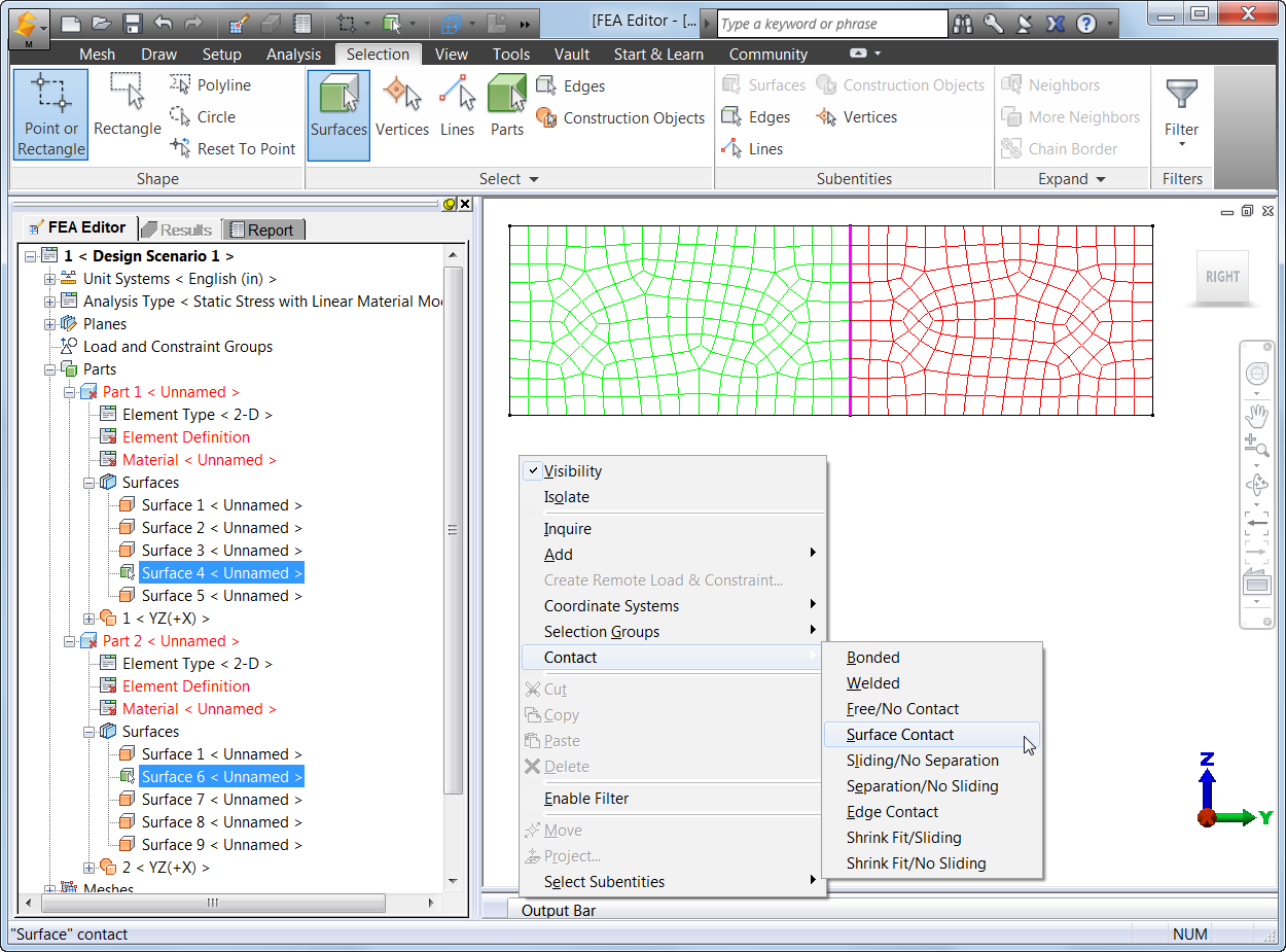
4. In the model display, select the coincident surfaces and right click. In the pop-up menu, choose "Contact" and then specify the type of contact from five applicable options (see Figure 2):
• Bonded - The nodes on the two edges will be matched and will be in perfect contact throughout the analysis. When a node on one edge deflects, the node on the adjoining edge will deflect the same amount in the same direction. This is the default option.
• Free/No Contact - The nodes on the two edges will not be matched and will be free to move relative to each other.
• Surface Contact - The nodes on the two edges will be matched and will be free to move away from each other. If the nodes move toward each other, a stiffness will be applied to resist this movement.

o   Sliding/No Separation – Bonds contact faces in normal to face direction while sliding under deformation.

o   Separation/No Sliding – Separates contact faces partially or fully without them sliding against each other.

Note that Edge Contact and Welded Contact are not applicable to 2D elements.

Figure 2: Once the mesh is generated, you can select and right click on the coincident surfaces and specify the type of contact.

4. After defining the type of contact, the contact surfaces will be listed in the tree view.
5. In the tree view, right click on the contact pair and choose "Settings..." (see Figure 3).

Figure 3: Right click on the contact pair in the tree view and choose "Settings...".

6. In the "Contact Options" dialog, you can specify the coefficient of friction for the contact pair (see Figure 4).

Figure 4: Choose whether or not to include friction in the analysis and specify the static friction coefficient.

7. Set up for linear static stress analysis (define element information, material properties, loadings and constraints) and run the analysis.
8. In the Results environment, you can inquire on the total contact force for each contact pair in the model. Right click on the heading for the contact pair in the tree view and choose the "Contact Force..." command (see Figure 5).

Figure 5: In Results environment, you can inquire on the total contact force. A "Total Contact Force" dialog will appear with the total contact force for that pair.

Thus, the ability to quickly and easily define 2-D contact helps you to perform linear static stress analysis of 2-D assembly models that were created with Autodesk Simulation’s sketching, modeling and meshing tools.